Parallelized cosmoTransitions Simulations¶

Preliminaries¶

For this tutorial, we’ll take advantage of a simple two scalar model included in the standard cosmoTransitions package for testing purposes. This model doesn’t have any physical significance. Instead, simply exists to test and highlight some of the features of the cosmoTransitions package. It consists of two scalar fields, labeled phi1 and phi2, which mix and an extra boson whose mass depends on both fields. There are six parameters used to characterize the potential of this model which are

• m1: Tree-level mass of phi1 when mu = 0
• m2: Tree-level mass of phi2 when mu = 0
• mu: Mass coefficient for the phi1-phi2 mixing term
• Y1: Coupling of the extra boson to the two scalars individually
• Y2: Coupling to the two scalars together
• n: Degrees of freedom of the extra boson

In what follows, we’ll perform a parallelized Monte Carlo simulation of the parameter space for this model.

Installing cosmoTransitions¶

By far, the easiest way to obtain cosmoTransitions is to directly clone the repository from github. To do this, simply log into titan and then cd to the place where you would like cosmoTransitions to be installed, e.g., in your home directory. Once there, type

git clone https://github.com/clwainwright/CosmoTransitions.git

If everything worked, there should be a new folder called CosmoTransitions. Since the cosmoTransitions package is simply a collection of python modules, it is now effectively installed and ready for use as long as you have previously installed python as described in First Steps.

The model file that we’ll use is in the CosmoTransitions/test folder and is called testModel1.py. We can perform a practice simulation of the phase history of this model for the default parameter values by creating a copy of this file in the CosmoTransitions folder and running it in an ipython shell. To do this, first, while in the CosmoTransitions folder, type cp test/testModel1.py . and then open an ipython shell by typing ipython at the terminal prompt. After this, perform the simulation by typing the following commands

from testModel1 import model1
m = model1()
alltrans = m.findAllTransitions()

This creates an instance of the model, runs cosmoTransitions, and saves the phase history in the variable alltrans. For the default parameters, this history includes two phase transitions which can be accessed by typing either alltrans[0] or alltrans[1]. Each of these is a python dictionary from which the information on the given transition can be extracted by referencing the appropriate key, e.g., typing alltrans[0]['trantype'], alltrans[1]['trantype'] will return (2,1) which indicates that the high (low) temperature transition was 2nd- (1st-) order. To exit the ipython shell just type exit. In the next subsection, we’ll see how to setup a Monte Carlo simulation of the parameter space using the titan cluster.

Setting up for Parallelized Simulation¶

To begin, in the CosmoTransitions folder create two folders, one named analysis and the other named data. Once this is done, cd into the analysis folder, open a text editor, copy/paste the following script into it

from pandas import DataFrame
from numpy.random import randint, uniform

def generate_points(num_points):

    def randN(initial_point, final_point, N, kind):
        if kind == 'integer':
            return randint(initial_point, final_point, size=N)
        if kind == 'float':
            return uniform(initial_point, final_point, size=N)

    df = DataFrame({'m1': randN(100, 150, num_points, 'float'),
                    'm2': randN(25, 75, num_points, 'float'),
                    'mu': randN(1, 50, num_points, 'float'),
                    'Y1': randN(.05, .25, num_points, 'float'),
                    'Y2': randN(.05, .25, num_points, 'float'),
                    'n': randN(10, 30, num_points, 'integer')})
    df = df[['m1', 'm2', 'mu', 'Y1', 'Y2', 'n']]

    return df

for cnt in range(5):
    points = generate_points(25)
    points.to_csv('../data/inputfile_%d.csv' % cnt, index=False, header=False)

and save it as generate_points.py. This script defines a function, generate_points, which generates num_points random choices for the six parameters in the scalar potential of our model. At the bottom of the script is a for loop which generates 5 separate files with 25 parameter points in each and exports them, in csv format, to the data folder. To run this, simply type python generate_points.py while in the analysis folder. If it ran correctly, then you should see 5 separate csv files in the data folder with 25 points in each.

Next, while still in the analysis folder, open a new text editor, copy/paste the following script into it

import sys
import pandas as pd
from pandas import DataFrame
from testModel1 import model1

jobPATH = sys.argv[1]
data = pd.read_csv(jobPATH + '/inputfile.csv')

trans_data = {}
for instance_count, instance in enumerate(data.values):
        m1, m2, mu, Y1, Y2, n = tuple(instance)
        m = model1(m1=m1, m2=m2, mu=mu, Y1=Y1, Y2=Y2, n=n)
        try:
                alltrans = m.findAllTransitions()
        except:
                continue
        else:
                alltrans = [x for x in alltrans if x is not None]
                if len(alltrans) > 0:
                        trans_dict = {}
                        for trans_count, trans in enumerate(alltrans):
                                try:
                                        trans_dict = {'Critical Temperature': trans['crit_trans']['Tcrit'],
                                                      'Nucleation Temperature': trans['Tnuc'],
                                                      'Action': trans['action'],
                                                      'phi1 High VEV': trans['high_vev'][0],
                                                      'phi1 Low VEV': trans['low_vev'][0],
                                                      'phi2 High VEV': trans['high_vev'][1],
                                                      'phi2 Low VEV': trans['low_vev'][1]}
                                except:
                                        continue

                        trans_data[instance_count] = {'m1': m1, 'm2': m2, 'mu': mu, 'Y1': Y1, 'Y2': Y2, 'n': n,
                                                        'Transition Info': trans_dict}

full_df = DataFrame(trans_data).transpose()
full_df = full_df.reset_index()
full_df.drop('index', axis=1, inplace=True)
full_df.to_csv(jobPATH + '/outputfile.csv', index=False)

and save it as runner.py. Given the correct path at runtime, this script will read a csv file of random parameter points, extract the phase history for each one, and output all the results to another csv file in the same path.

By running runner.py on each of the 5x25=125 parameter points, we can scan the phase history of this model as a function of the full parameter space. However, by setting up 5 separate instances of it which simultaneously run on one of the 5 csv files created by generate_points.py, we can reduce our running time by roughly 1/5. In the next subsection, this is what we’ll do.

Parallelized Simulation¶

So far, in the CosmoTransitions folder, there is an analysis folder and a data folder. The analysis folder should contain both generate_points.py and runner.py and the data folder should contain 5 csv files. Now, while in the CosmoTransitions folder, open a text editor, copy and paste the following script into it

#/bin/sh

# Define some paths
cosmoBase="$HOME/CosmoTransitions"
cosmoDataBase=$cosmoBase"/data"
cosmoAnalysisBase=$cosmoBase"/analysis"
cosmoJobBase=$cosmoBase"/jobs"

# Create folder to run jobs and cd into it
mkdir $cosmoJobBase
cd $cosmoJobBase

# Get number of data inputfiles
numfiles=($cosmoDataBase/*)
numfiles=${#numfiles[@]}

# Begin loop
for (( i=0; i<$numfiles; i++ ));
do

# Define a folder for a job and cp all necessary files to this location
JobBase=$cosmoJobBase"/job$i"
mkdir $JobBase
cp -r $cosmoBase"/cosmoTransitions" $cosmoAnalysisBase"/runner.py" $cosmoBase"/test/testModel1.py" $JobBase
cp $cosmoDataBase"/inputfile_$i.csv" $JobBase"/inputfile.csv"
cd $JobBase

# Create a bash script for batch submission
################################################################
echo "" >> bout.log
echo "" >> berr.log

echo "#!/bin/bash" >> script.sh
echo "#PBS -N Job$i" >> script.sh
echo "echo 'seed: $i'" >> script.sh
echo "printenv" >> script.sh
echo "" >> script.sh
echo 'echo "Running cosmoTransitions"' >> script.sh
echo "PYTHONPATH=$HOME/local/anaconda/lib/python2.7/site-packages $HOME/local/anaconda/bin/python $JobBase/runner.py $JobBase" >> script.sh
################################################################


# Submit bash script
chmod +x script.sh
qsub -e berr.log -o bout.log script.sh

# Exit loop
done

and save it as run_cosmo_jobs. As before, make it an executable with chmod +x run_cosmo_jobs. run_cosmo_jobs creates five folders with each containing one of the csv files created by generate_points.py, a copy of runner.py, a copy of the cosmoTransitions package, our model file, and a bash script. This bash script submits a job to the titan cluster which consists of running the local version of runner.py on the given csv file. The qsub cmd is what submits this job to cluster instead of running it locally.

Now, if everything has been setup correctly, then you should be able to perform parallel Monte Carlo simulations of the parameter space by running the previous script as ./run_cosmo_jobs from the CosmoTransitions folder. If everything worked correctly, you should see output similar to the following

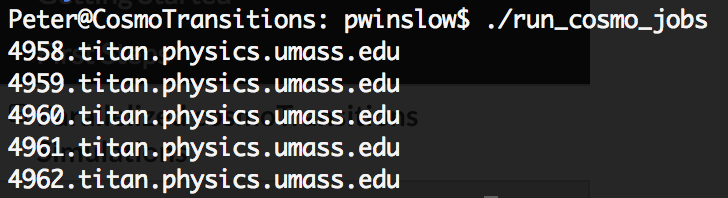
Your jobs should now be running on the titan cluster. While they’re running, you can check on them using the qstat cmd which should return output similar to the following

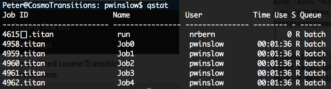
For more interface options with running jobs, see any of the links here.

Cleanup and Results¶

After your jobs have finished running, i.e., they no longer appear when you run qstat, you’ll have five output.csv files containing the results which are spread out among the five folders job0, job1, etc. These can be all combined again with a short bash script. To do this, from the CosmoTransitions folder, copy and paste the following script into a new file

#/bin/sh

# Define some paths
cosmoBase="$HOME/CosmoTransitions"
cosmoDataBase=$cosmoBase"/data"
cosmoJobBase=$cosmoBase"/jobs"

# Get number of data inputfiles
numfiles=($cosmoDataBase/*)
numfiles=${#numfiles[@]}

# Define the overall output csv file
outputFile=$cosmoDataBase"/output.csv"

# Begin loop
for (( i=0; i<$numfiles; i++ ));
do

JobBase=$cosmoJobBase"/job$i"
cat $JobBase"/outputfile.csv" >> $outputFile

done

save it as clean_cosmo_jobs and make it an executable. Running this script will combine all five csv files returned by titan into a single output.csv file which is then stored in the data folder for further analysis. We can explore the results stored in this output.csv file by opening an ipython shell from the data folder. The following shows a number of commands that can be used to understand and access the results

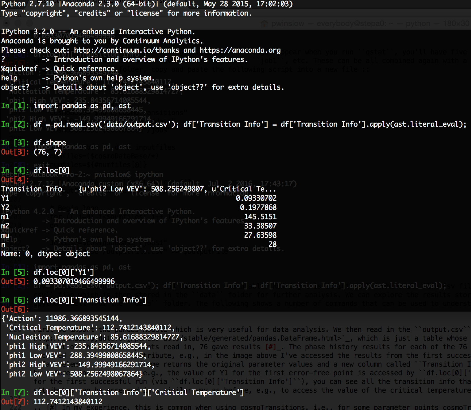
First we import the pandas module which is very useful for data analysis. We then read in the output.csv file in the form of a pandas dataframe, which is just a table whose rows and columns are labeled. We then see that out of the 5x25=125 points read in, 76 gave results [1]. The phase history results for each of the 76 successful cosmoTransitions runs can be accessed via the loc attribute, e.g., in the image above I’ve accessed the results from the first successful cosmoTransitions run using df.loc[0]. Each element of the dataframe returns the original parameter values and a new column called Transition Info. The parameter values can be accessed by referencing their name, e.g., the value of Y1 for the first successful run is accessed by df.loc[0]['Y1']. By referencing the transition info for the first successful run (via df.loc[0]['Transition Info']), you can see all the transition info that was stored for each run. These transition attributes can be accessed in a similar way as before, e.g., to access the value of the critical temperature you can use df.loc[0]['Transition Info']['Critical Temperature'].

Final Comments¶

This concludes the tutorial on how to perform distributed Monte Carlo simulations of a cosmoTransitions model on the titan cluster. In order to expand on this for your own research, you’ll just need to repeat the above procedure with

• your own model file
• your own generate_points.py (this should be modified based on the free parameters of your own model and their bounds)
• your own runner.py (this should be modified based on the free parameters of your own model)

If you have any questions or problems with the above procedure, feel free to contact me.